Search

Using Regression SVM to Solve Regression Problems

The SVM task trains a Support Vector Machine for regression. The SVM model uses a kernel function (a generalization of scalar product) to find the optimal separating surfaces in data.

The output of the task is a model, containing a weight matrix w_ji ,that can be employed by the Apply Model task to perform the SVM forecast on a set of examples.

Prerequisites

a Rulex process has been created
the required datasets have been imported into the process
the data used for the model has been well prepared, and contains a categorical output and a number of inputs.
a single unified dataset has been created by merging all the datasets imported into the process.

Additional tabs

Along with the Options tab, where the task can be configured, the following additional tabs are provided:

Documentation tab where you can document your task,
Parametric options tab where you can configure process variables instead of fixed values. Parametric equivalents are expressed in italics in this page (PO).
Monitor and results tabs, where you can see the output of the task computation. See Results table below.

Procedure

Drag and drop the Regression SVM task onto the stage.
Connect a task, which contains the attributes from which you want to create the model, to the new task.
Double click the Regression SVM task.
Configure the options described in the table below.
Save and compute the task.

Parameter Name	PO	Description
Regression SVM options
SVM formulation	svmtype	Select the formulation for the SVM problem. Possible choices are: EPSILON_SVR: this formulation uses the epsilon parameter, through which it is possible to check the error percentage of the model. NU_SVC: this formulation uses the nu parameter to check the fraction of examples used as support vectors.
Gamma in kernel function	svmgamma	Specify the value of the parameter γ in the kernel function. Note this parameter is only required for Polynominal, Radial basis function and Sigmoid kernel functions.
Kernel function	svmkernel	Indicate the kernel function to be used. Possible choices are: Linear: K(x_{i ,}x_j) = x_i . x_j Polynominal: K(x_{i ,}x_j) = (γx_i . xj + C₀)^d Radial basis function: K(x_{i ,}x_j) = exp(-γ\|\|x_i - x_j\|\|²) Sigmoid: K(x_{i ,}x_j) = tanh(γx_i . xj + C₀)
Coef0 in kernel function	svmcoeff0	Specify the value of the parameter c₀ in the kernel function. Note this parameter is only required for Polynominal and Sigmoid kernel functions.
Degree in kernel function	svmdegree	Specify the value of the parameter d in the kernel function. Note this parameter is only required for Polynominal kernel functions.
Parameter C	svmcost	Specify the value of the parameter C in the SVM formulation.
Normalization for input variables	normtype	The type of normalization to use when treating ordered (discrete or continuous) variables. Possible methods are: None: no normalization is performed (default) Normal: data are normalized according to the Gaussian distribution, where μ is the average of x and σ is its standard deviation: Minmax [0,1]: data are normalized to be comprised in the range [0,1]: Minmax [-1, 1]: data are normalized to be included in the range [-1, 1]: Every attribute can have its own value for this option, which can be set in the Data Manager task. These choices are preserved if Attribute is selected in the Normalization of input variables option; otherwise any selections made here overwrite previous selections made.
Parameter epsilon of epsilon-SVR	svmeps	The ε parameter allows the user to control the number of possible errors in the training set: the higher the number, the higher the number of errors allowed.
Use shrinking heuristics	svmshrinking	If selected, heuristic methods will be used to speed up computation.
Parameter nu of nu-SVC	svmnu	Specify the value of the parameter ν in the nv-SVM formulation. The ν parameter, which must range from 0 to 1, is related to the fraction of examples used as support vectors.
Aggregate data before processing	aggregate	If selected, identical patterns are aggregated and considered as a single pattern during the training phase.
Tolerance threshold	svmtol	Specify the tolerance of the terminating criterion.
Append results	append	If selected, the results of this computation are appended to the dataset, otherwise they replace the results of previous computations.
Cache memory size	svmcachesize	Specify the amount of cache that can be used during training.
Input attributes	inpnames	Drag and drop the input attributes you want to use for the classification of data.
Output attributes	outnames	Drag and drop the attributes you want to use to form the final classes into which the dataset will be divided.

Results

The results of the SVM task can be viewed in two separate tabs:

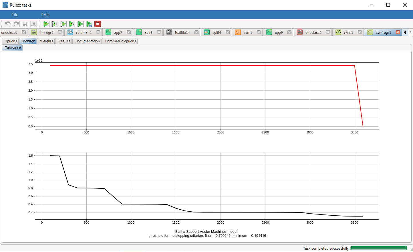
The Monitor tab, where it is possible to view the temporal evolution of some quantities related to the SVM optimization during its execution. In particular, the behavior of tolerance, and its minimum is reported as a function of the number of iterations. These plots can be viewed during and after computation operations.
The Results tab, where statistics on the SVM computation are displayed, such as the execution time, number of attributes etc..

Example

The following examples are based on the Adult dataset.

Scenario data can be found in the Datasets folder in your Rulex installation.

The scenario aims to solve a simple regression problem based on the hours per week people statistically work, according to such factors as their age, occupation and marital status.

The following steps were performed:

First we import the adult dataset with an Import from Text File task.
Split the dataset into a test and training set with a Split Data task.
Generate the model from the dataset with the SVM task.
Apply the model to the dataset with an Apply Model task, to forecast the output associated with each pattern of the dataset.
Use the Take a Look functionality to check the results of the computation.

Procedure	Screenshot
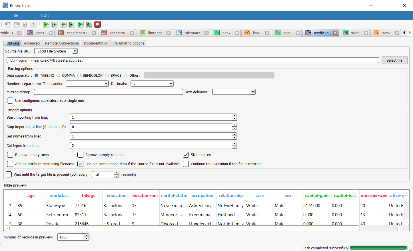
Import the adult dataset with the Import from Text File task, and take the data types from line 2.
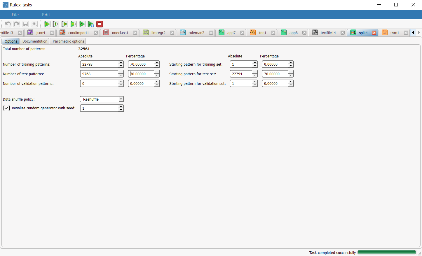
Split the dataset into test and training sets (30% test and 70% training) with the Split Data task.
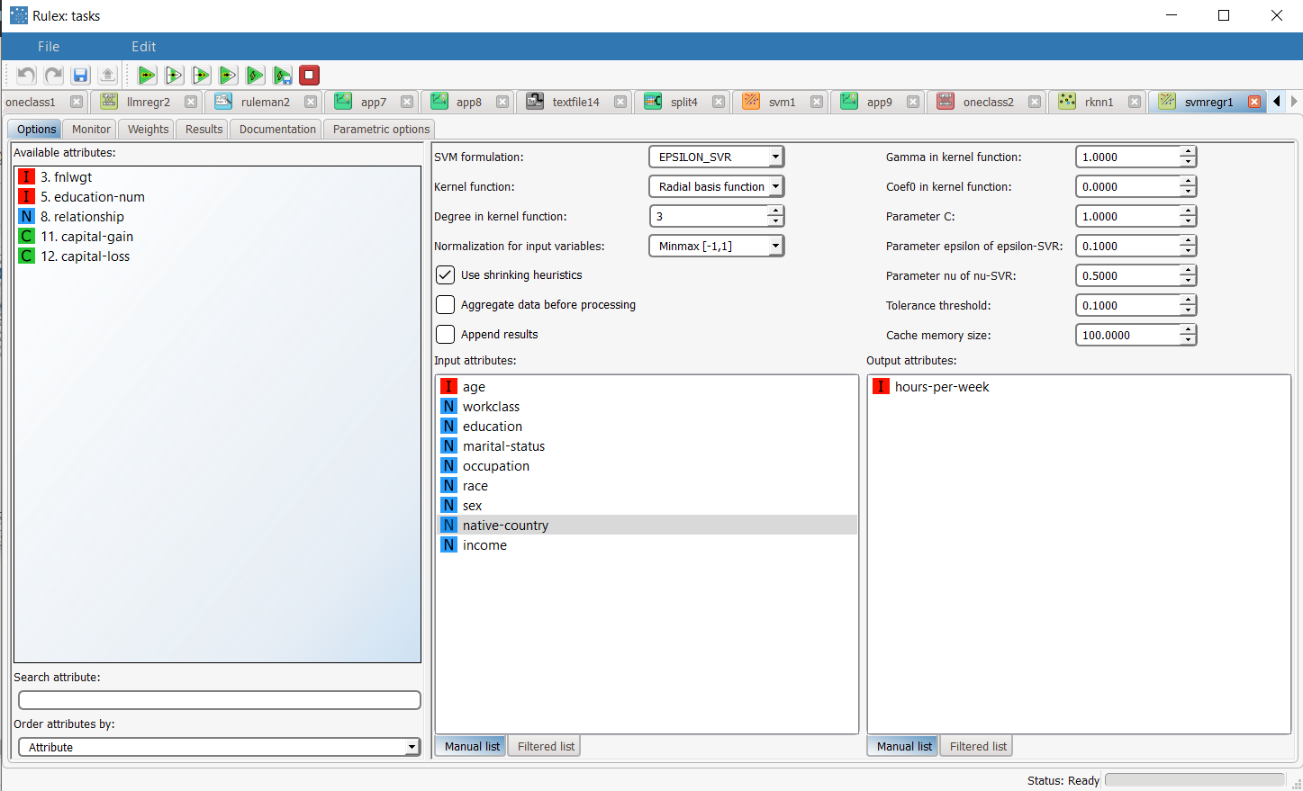
Add an SVM Regression task to the process and double click the task. Maintaining the default SVM settings, compute the task. Drag and drop the hours-per-week attribute onto the Output Attributes edit box, then the following attributes as input attributes: age workclass education occupation race sex native-country income.	Note that this regression problem in completely different from the SVM classification problem, where income was the output. In this regression example, we are not particularly interested in the physical meaning of this analysis, but only want to illustrate the potentiality of regression in a real-world dataset.
The execution of the SVM task can be viewed in the Monitor tab. In these plots the behavior of the tolerance (and its minimum) as a function of the iteration is showed.
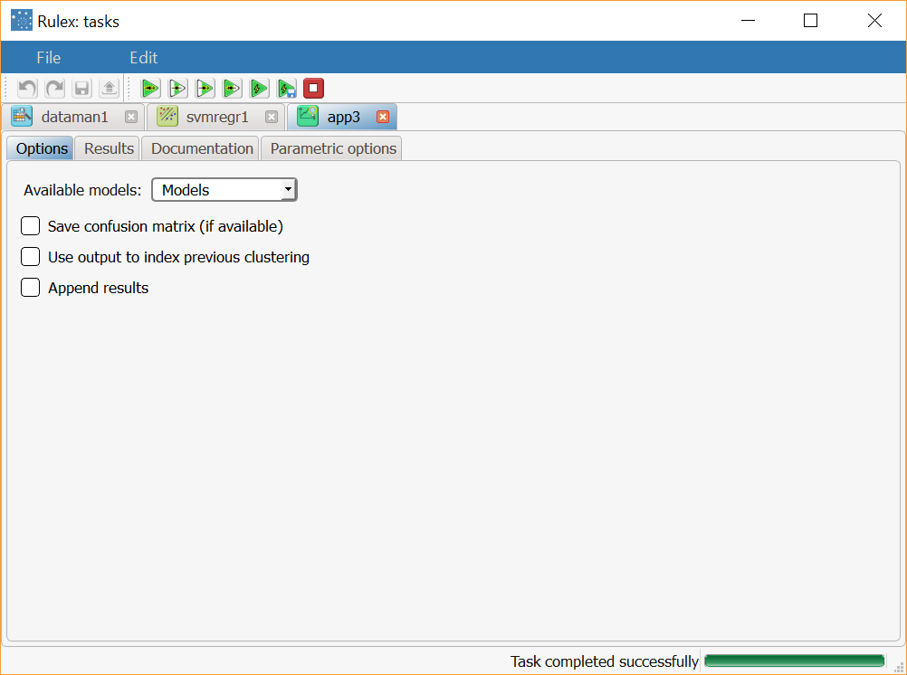
The forecast ability of the set of the generated model can be viewed by adding an Apply Model task to the SVM task, and computing with default options.
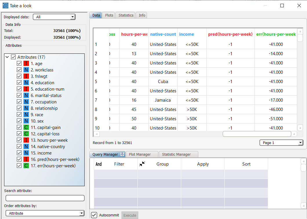
To see the results, right-click the Apply Model task and select Take a look. In the data table the following columns relative to the results of SVM elaboration have been added: the pred(hours-per-week) column contains the output forecast generated by the SVM model. the err(hours-per-week) column contains the error, which corresponds to the difference between the predicted output and the real one. If the actual output is missing, this field is also left empty.